PyTorch: Part 2 - Autograd, Automatic Gradients

What is Autograd?

In Part 1, we learned about tensors. Now it’s time to learn about Autograd, PyTorch’s automatic differentiation engine.

Autograd automatically calculates gradients (derivatives) for you. This is essential for training neural networks.

Don’t worry if gradients sound scary. Let’s break it down with a simple example.

---

A Simple Example

Let’s say we have a function: y = x²

If x = 3, then y = 9.

Now, gradient (or derivative) tells us: “If we change x a little bit, how much does y change?”

For y = x², the gradient is dy/dx = 2x.

So when x = 3, the gradient is 2 × 3 = 6.

This means if we increase x by 1, y increases by about 6.

---

Tracking Gradients in PyTorch

To make PyTorch track gradients, we use requires_grad=True:

import torch

# Create a tensor and tell PyTorch to track operations
x = torch.tensor(3.0, requires_grad=True)
print(f"x = {x}")

# Perform some operation
y = x ** 2  # y = x²
print(f"y = {y}")

# Calculate gradients
y.backward()

# Access the gradient
print(f"dy/dx = {x.grad}")  # Should be 2*x = 6

Output:

x = tensor(3., requires_grad=True)
y = tensor(9., grad_fn=<PowBackward0>)
dy/dx = tensor(6.)

Let’s break down what happened:

1. We created x with requires_grad=True to tell PyTorch to track all operations
2. We calculated y = x²
3. We called y.backward() to compute gradients
4. We accessed the gradient with x.grad

That’s it! PyTorch figured out that dy/dx = 6 automatically.

---

The Computation Graph

When you do operations on tensors with requires_grad=True, PyTorch builds a computation graph behind the scenes.

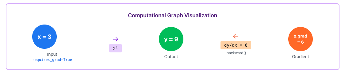
The forward pass goes left to right (calculating y from x). The backward pass goes right to left (calculating gradients).

Notice how y has grad_fn=<PowBackward0>. This tells PyTorch which operation created this tensor, so it knows how to calculate gradients.

---

A More Complex Example

Let’s try a function with multiple variables:

# Multiple operations
x = torch.tensor(2.0, requires_grad=True)
y = torch.tensor(3.0, requires_grad=True)

# Function: z = x² + 2xy + y²
z = x**2 + 2*x*y + y**2
print(f"z = {z}")

# Calculate all gradients at once
z.backward()

print(f"dz/dx = {x.grad}")  # Should be 2x + 2y = 10
print(f"dz/dy = {y.grad}")  # Should be 2x + 2y = 10

Output:

z = tensor(25., grad_fn=<AddBackward0>)
dz/dx = tensor(10.)
dz/dy = tensor(10.)

PyTorch automatically figured out both gradients. This is super powerful because real neural networks have millions of parameters!

---

Important Things to Know

Gradients Accumulate

One thing that trips up beginners is that gradients accumulate. If you call backward() multiple times, gradients add up:

x = torch.tensor(2.0, requires_grad=True)

# First calculation
y = x ** 2
y.backward()
print(f"After first backward: {x.grad}")  # 4

# Second calculation
y = x ** 2
y.backward()
print(f"After second backward: {x.grad}")  # 8 (4 + 4)

To fix this, always reset gradients before each backward pass:

x.grad.zero_()  # Reset gradient to 0

Disabling Gradient Tracking

Sometimes you don’t want PyTorch to track gradients (like during inference). Use torch.no_grad():

x = torch.tensor(2.0, requires_grad=True)

# With gradient tracking
y = x ** 2
print(y.requires_grad)  # True

# Without gradient tracking
with torch.no_grad():
    y = x ** 2
    print(y.requires_grad)  # False

This saves memory and speeds up computation.

Detaching Tensors

You can also detach a tensor from the computation graph:

x = torch.tensor(2.0, requires_grad=True)
y = x ** 2

# Detach y from the graph
z = y.detach()
print(z.requires_grad)  # False

---

Practical Example: Finding the Minimum

Let’s use gradients to find the minimum of a function. We’ll find where f(x) = (x - 5)² is minimum (which is at x = 5).

# Start at x = 0
x = torch.tensor(0.0, requires_grad=True)
learning_rate = 0.1

for i in range(20):
    # Forward pass
    y = (x - 5) ** 2

    # Backward pass
    y.backward()

    # Update x (gradient descent)
    with torch.no_grad():
        x -= learning_rate * x.grad

    # Reset gradient
    x.grad.zero_()

    if i % 5 == 0:
        print(f"Step {i}: x = {x.item():.3f}, f(x) = {y.item():.3f}")

print(f"\nFinal: x = {x.item():.3f} (should be close to 5)")

Output:

Step 0: x = 1.000, f(x) = 25.000
Step 5: x = 3.672, f(x) = 1.762
Step 10: x = 4.537, f(x) = 0.214
Step 15: x = 4.849, f(x) = 0.023

Final: x = 4.950 (should be close to 5)

We just implemented gradient descent! The gradient tells us which direction to move, and we slowly approach the minimum.

---

Quick Reference

Concept	What It Does
requires_grad=True	Tell PyTorch to track operations on this tensor
.backward()	Compute gradients
.grad	Access the computed gradient
.grad.zero_()	Reset gradient to zero
torch.no_grad()	Context manager to disable gradient tracking
.detach()	Create a copy not connected to computation graph
grad_fn	Shows which operation created the tensor

---

Key Takeaways

• Autograd automatically calculates gradients (derivatives)
• Use requires_grad=True to track operations
• Call .backward() to compute gradients
• Access gradients with .grad
• Always reset gradients before each backward pass with .grad.zero_()
• Use torch.no_grad() during inference to save memory
• This is the foundation for training neural networks

---

What’s Next?

Now that we understand tensors and autograd, we’re ready to build Neural Networks in Part 3. We’ll learn how to use torch.nn to create layers and models.

See you in Part 3!