PyTorch: Part 3 - Building Neural Networks

What is a Neural Network?

In Part 1 we learned about tensors, and in Part 2 we learned about autograd. Now let’s put them together to build neural networks.

A neural network is basically a mathematical function with adjustable parameters (called weights and biases). We adjust these parameters during training to make better predictions.

Think of it like this:

Input → Hidden Layers → Output

Each layer applies a transformation: output = activation(weights × input + bias)

---

The nn.Module Class

In PyTorch, we build neural networks by creating a class that inherits from nn.Module.

Here’s the basic structure:

import torch
import torch.nn as nn

class SimpleNet(nn.Module):
    def __init__(self):
        super(SimpleNet, self).__init__()
        # Define layers here

    def forward(self, x):
        # Define how data flows through layers
        return x

Two important things:

1. __init__: Define all your layers here
2. forward: Define how data flows through the layers

---

Building Our First Network

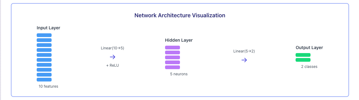
Let’s build a simple network with:

• Input: 10 features
• Hidden layer: 5 neurons
• Output: 2 classes

import torch
import torch.nn as nn

class SimpleNet(nn.Module):
    def __init__(self):
        super(SimpleNet, self).__init__()
        # Linear layer: input_features → output_features
        self.fc1 = nn.Linear(10, 5)   # 10 inputs → 5 outputs
        self.fc2 = nn.Linear(5, 2)    # 5 inputs → 2 outputs

    def forward(self, x):
        # x goes through first layer with ReLU activation
        x = torch.relu(self.fc1(x))
        # Then through second layer
        x = self.fc2(x)
        return x

# Create the network
model = SimpleNet()
print(model)

Output:

SimpleNet(
  (fc1): Linear(in_features=10, out_features=5, bias=True)
  (fc2): Linear(in_features=5, out_features=2, bias=True)
)

We just created a neural network! Here’s what it looks like:

Let’s break down what each part does.

---

Understanding Linear Layers

nn.Linear(in_features, out_features) is the most common layer type. It’s also called a fully connected layer or dense layer.

What it does:

output = input × weights + bias

For nn.Linear(10, 5):

• Takes input with 10 features
• Produces output with 5 features
• Has 10×5 = 50 weights + 5 biases = 55 parameters

# Check the number of parameters
layer = nn.Linear(10, 5)
print(f"Weights shape: {layer.weight.shape}")   # [5, 10]
print(f"Bias shape: {layer.bias.shape}")        # [5]
print(f"Total parameters: {layer.weight.numel() + layer.bias.numel()}")  # 55

---

Activation Functions

Activation functions add non linearity to our network. Without them, stacking multiple linear layers would just be one big linear function.

ReLU (Most Common)

ReLU is simple: if the value is negative, make it 0. Otherwise, keep it.

x = torch.tensor([-1.0, 0.0, 1.0, 2.0])
relu = torch.relu(x)
print("ReLU:", relu)  # tensor([0., 0., 1., 2.])

Sigmoid (Output 0 to 1)

Good for probabilities or binary classification.

x = torch.tensor([-1.0, 0.0, 1.0])
sigmoid = torch.sigmoid(x)
print("Sigmoid:", sigmoid)  # tensor([0.2689, 0.5000, 0.7311])

Softmax (For Classification)

Converts scores to probabilities that sum to 1.

logits = torch.tensor([2.0, 1.0, 0.1])
softmax = torch.softmax(logits, dim=0)
print("Softmax:", softmax)  # tensor([0.6590, 0.2424, 0.0986])
print("Sum:", softmax.sum())  # tensor(1.)

---

The Forward Pass

The forward method defines how data flows through the network.

model = SimpleNet()

# Create random input (batch_size=3, features=10)
x = torch.randn(3, 10)
print("Input shape:", x.shape)

# Forward pass
output = model(x)
print("Output shape:", output.shape)
print("Output:\n", output)

Output:

Input shape: torch.Size([3, 10])
Output shape: torch.Size([3, 2])
Output:
 tensor([[-0.3456,  0.2134],
        [ 0.1234, -0.5678],
        [-0.2341,  0.4567]], grad_fn=<AddmmBackward0>)

Notice:

• We put in 3 samples with 10 features each
• We got out 3 samples with 2 values each (our 2 classes)
• The output has grad_fn because PyTorch is tracking gradients

---

Common Layer Types

Here are other layer types you’ll encounter:

Convolutional Layer (for images)

# For image processing
conv = nn.Conv2d(in_channels=3, out_channels=16, kernel_size=3)

Dropout (prevents overfitting)

# Randomly sets 50% of neurons to 0 during training
dropout = nn.Dropout(p=0.5)

Batch Normalization (stabilizes training)

# Normalizes layer outputs
bn = nn.BatchNorm1d(num_features=5)

---

Checking Model Parameters

You can see all trainable parameters:

model = SimpleNet()

# Count parameters
total_params = sum(p.numel() for p in model.parameters())
print(f"Total parameters: {total_params}")

# See all parameters
for name, param in model.named_parameters():
    print(f"{name}: {param.shape}")

Output:

Total parameters: 67
fc1.weight: torch.Size([5, 10])
fc1.bias: torch.Size([5])
fc2.weight: torch.Size([2, 5])
fc2.bias: torch.Size([2])

---

Training vs Evaluation Mode

Neural networks behave differently during training and evaluation. Some layers like Dropout and BatchNorm act differently.

model = SimpleNet()

# Training mode (default)
model.train()
print(model.training)  # True

# Evaluation mode
model.eval()
print(model.training)  # False

---

Moving Model to GPU

If you have a GPU, you can speed up training:

# Check if GPU is available
device = torch.device('cuda' if torch.cuda.is_available() else 'cpu')
print(f"Using device: {device}")

# Move model to GPU
model = SimpleNet()
model = model.to(device)

# Don't forget to move data too!
x = torch.randn(3, 10).to(device)
output = model(x)

---

Quick Reference

Method	What It Does
model.parameters()	Returns all trainable parameters
model.train()	Set to training mode
model.eval()	Set to evaluation mode
model.to(device)	Move model to CPU or GPU
model.state_dict()	Get all parameters as dictionary
model.load_state_dict()	Load saved parameters

---

Key Takeaways

• Build networks by inheriting from nn.Module
• Define layers in __init__, use them in forward
• nn.Linear is the basic fully connected layer
• ReLU is the most common activation function
• Use model.train() for training, model.eval() for inference
• Always use model(x) not model.forward(x)
• Move model and data to GPU with .to(device)

---

What’s Next?

We now know how to build neural networks. But how do we actually train them? In Part 4, we’ll learn about the Training Loop. We’ll cover:

• Loss functions
• Optimizers
• The complete training loop
• Making predictions

See you in Part 4!